Directory:Jon Awbrey/Papers/Differential Logic

Note 1

One of the first things that you can do, once you have a really decent calculus for boolean functions or propositional logic, whatever you want to call it, is to compute the differentials of these functions or propositions.

Now there are many ways to dance around this idea, and I feel like I have tried them all, before one gets down to acting on it, and there many issues of interpretation and justification that we will have to clear up after the fact, that is, before we can be sure that it all really makes any sense, but I think this time I'll just jump in, and show you the form in which this idea first came to me.

Start with a proposition of the form \(x ~\operatorname{and}~ y,\) which is graphed as two labels attached to a root node:

o---------------------------------------o | | | x y | | @ | | | o---------------------------------------o | x and y | o---------------------------------------o

Written as a string, this is just the concatenation "\(x~y\)".

The proposition \(xy\!\) may be taken as a boolean function \(f(x, y)\!\) having the abstract type \(f : \mathbb{B} \times \mathbb{B} \to \mathbb{B},\) where \(\mathbb{B} = \{ 0, 1 \}\) is read in such a way that \(0\!\) means \(\operatorname{false}\) and \(1\!\) means \(\operatorname{true}.\)

In this style of graphical representation, the value \(\operatorname{true}\) looks like a blank label and the value \(\operatorname{false}\) looks like an edge.

o---------------------------------------o | | | | | @ | | | o---------------------------------------o | true | o---------------------------------------o

o---------------------------------------o | | | o | | | | | @ | | | o---------------------------------------o | false | o---------------------------------------o

Back to the proposition \(xy.\!\) Imagine yourself standing in a fixed cell of the corresponding venn diagram, say, the cell where the proposition \(xy\!\) is true, as shown here:

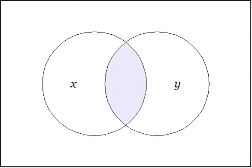
Now ask yourself: What is the value of the proposition \(xy\!\) at a distance of \(dx\!\) and \(dy\!\) from the cell \(xy\!\) where you are standing?

Don't think about it — just compute:

o---------------------------------------o | | | dx o o dy | | / \ / \ | | x o---@---o y | | | o---------------------------------------o | (x + dx) and (y + dy) | o---------------------------------------o

To make future graphs easier to draw in ASCII, I will use devices like @=@=@ and o=o=o to identify several nodes into one, as in this next redrawing:

o---------------------------------------o | | | x dx y dy | | o---o o---o | | \ | | / | | \ | | / | | \| |/ | | @=@ | | | o---------------------------------------o | (x + dx) and (y + dy) | o---------------------------------------o

However you draw it, these expressions follow because the expression \(x + dx,\!\) where the plus sign indicates addition in \(\mathbb{B},\) that is, addition modulo 2, and thus corresponds to the exclusive disjunction operation in logic, parses to a graph of the following form:

o---------------------------------------o | | | x dx | | o---o | | \ / | | @ | | | o---------------------------------------o | x + dx | o---------------------------------------o

Next question: What is the difference between the value of the proposition \(xy\!\) "over there" and the value of the proposition \(xy\!\) where you are, all expressed as general formula, of course? Here 'tis:

o---------------------------------------o | | | x dx y dy | | o---o o---o | | \ | | / | | \ | | / | | \| |/ x y | | o=o-----------o | | \ / | | \ / | | \ / | | \ / | | \ / | | \ / | | @ | | | o---------------------------------------o | ((x + dx) & (y + dy)) - xy | o---------------------------------------o

Oh, I forgot to mention: Computed over \(\mathbb{B},\) plus and minus are the very same operation. This will make the relationship between the differential and the integral parts of the resulting calculus slightly stranger than usual, but never mind that now.

Last question, for now: What is the value of this expression from your current standpoint, that is, evaluated at the point where \(xy\!\) is true? Well, substituting \(1\!\) for \(x\!\) and \(1\!\) for \(y\!\) in the graph amounts to the same thing as erasing those labels:

o---------------------------------------o | | | dx dy | | o---o o---o | | \ | | / | | \ | | / | | \| |/ | | o=o-----------o | | \ / | | \ / | | \ / | | \ / | | \ / | | \ / | | @ | | | o---------------------------------------o | ((1 + dx) & (1 + dy)) - 1·1 | o---------------------------------------o

And this is equivalent to the following graph:

o---------------------------------------o | | | dx dy | | o o | | \ / | | o | | | | | @ | | | o---------------------------------------o | dx or dy | o---------------------------------------o

Note 2

We have just met with the fact that the differential of the and is the or of the differentials.

\(x ~\operatorname{and}~ y \quad \xrightarrow{~\operatorname{Diff}~} \quad dx ~\operatorname{or}~ dy\)

o---------------------------------------o | | | dx dy | | o o | | \ / | | o | | x y | | | @ --Diff--> @ | | | o---------------------------------------o | x y --Diff--> ((dx)(dy)) | o---------------------------------------o

It will be necessary to develop a more refined analysis of that statement directly, but that is roughly the nub of it.

If the form of the above statement reminds you of De Morgan's rule, it is no accident, as differentiation and negation turn out to be closely related operations. Indeed, one can find discussions of logical difference calculus in the Boole–De Morgan correspondence and Peirce also made use of differential operators in a logical context, but the exploration of these ideas has been hampered by a number of factors, not the least of which being a syntax adequate to handle the complexity of expressions that evolve.

For my part, it was definitely a case of the calculus being smarter than the calculator thereof. The graphical pictures were catalytic in their power over my thinking process, leading me so quickly past so many obstructions that I did not have time to think about all of the difficulties that would otherwise have inhibited the derivation. It did eventually became necessary to write all this up in a linear script, and to deal with the various problems of interpretation and justification that I could imagine, but that took another 120 pages, and so, if you don't like this intuitive approach, then let that be your sufficient notice.

Let us run through the initial example again, this time attempting to interpret the formulas that develop at each stage along the way.

We begin with a proposition or a boolean function \(f(x, y) = xy.\!\)

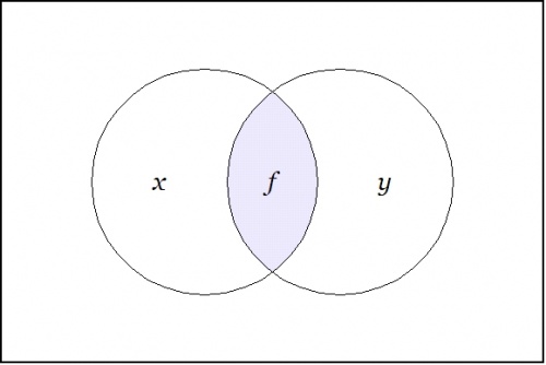
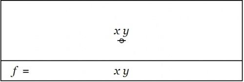
A function like this has an abstract type and a concrete type. The abstract type is what we invoke when we write things like \(f : \mathbb{B} \times \mathbb{B} \to \mathbb{B}\) or \(f : \mathbb{B}^2 \to \mathbb{B}.\) The concrete type takes into account the qualitative dimensions or the "units" of the case, which can be explained as follows.

Let \(X\!\) be the set of values \(\{ \texttt{(} x \texttt{)},~ x \} ~=~ \{ \operatorname{not}~ x,~ x \}.\)

Let \(Y\!\) be the set of values \(\{ \texttt{(} y \texttt{)},~ y \} ~=~ \{ \operatorname{not}~ y,~ y \}.\)

Then interpret the usual propositions about \(x, y\!\) as functions of the concrete type \(f : X \times Y \to \mathbb{B}.\)

We are going to consider various operators on these functions. Here, an operator \(\operatorname{F}\) is a function that takes one function \(f\!\) into another function \(\operatorname{F}f.\)

The first couple of operators that we need to consider are logical analogues of those that occur in the classical finite difference calculus, namely:

The difference operator \(\Delta,\!\) written here as \(\operatorname{D}.\)

The enlargement" operator \(\Epsilon,\!\) written here as \(\operatorname{E}.\)

These days, \(\operatorname{E}\) is more often called the shift operator.

In order to describe the universe in which these operators operate, it is necessary to enlarge the original universe of discourse, passing from the space \(U = X \times Y\) to its differential extension, \(\operatorname{E}U,\) that has the following description:

\(\operatorname{E}U ~=~ U \times \operatorname{d}U ~=~ X \times Y \times \operatorname{d}X \times \operatorname{d}Y,\)

with

\(\operatorname{d}X = \{ \texttt{(} \operatorname{d}x \texttt{)}, \operatorname{d}x \}\)  and  \(\operatorname{d}Y = \{ \texttt{(} \operatorname{d}y \texttt{)}, \operatorname{d}y \}.\)

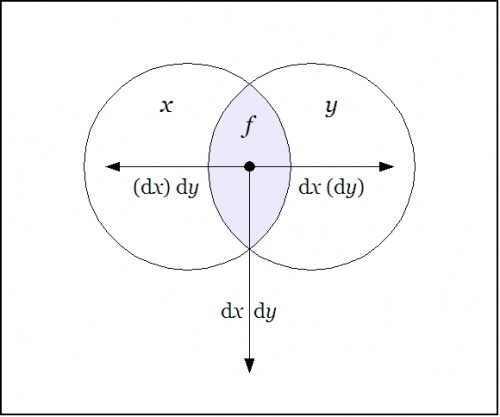
The interpretations of these new symbols can be diverse, but the easiest option for now is just to say that \(\operatorname{d}x\) means "change \(x\!\)" and \(\operatorname{d}y\) means "change \(y\!\)". To draw the differential extension \(\operatorname{E}U\) of our present universe \(U = X \times Y\) as a venn diagram, it would take us four logical dimensions \(X, Y, \operatorname{d}X, \operatorname{d}Y,\) but we can project a suggestion of what it's about on the universe \(X \times Y\) by drawing arrows that cross designated borders, labeling the arrows as \(\operatorname{d}x\) when crossing the border between \(x\!\) and \(\texttt{(} x \texttt{)}\) and as \(\operatorname{d}y\) when crossing the border between \(y\!\) and \(\texttt{(} y \texttt{)},\) in either direction, in either case.

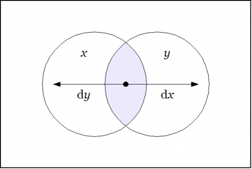
Propositions can be formed on differential variables, or any combination of ordinary logical variables and differential logical variables, in all the same ways that propositions can be formed on ordinary logical variables alone. For instance, the proposition \(\texttt{(} \operatorname{d}x \texttt{(} \operatorname{d}y \texttt{))}\) may be read to say that \(\operatorname{d}x \Rightarrow \operatorname{d}y,\) in other words, there is "no change in \(x\!\) without a change in \(y\!\)".

Given the proposition \(f(x, y)\!\) in \(U = X \times Y,\) the (first order) enlargement of \(f\!\) is the proposition \(\operatorname{E}f\) in \(\operatorname{E}U\) that is defined by the formula \(\operatorname{E}f(x, y, \operatorname{d}x, \operatorname{d}y) = f(x + \operatorname{d}x, y + \operatorname{d}y).\)

Applying the enlargement operator \(\operatorname{E}\) to the present example, \(f(x, y) = xy,\!\) we may compute the result as follows:

\(\operatorname{E}f(x, y, \operatorname{d}x, \operatorname{d}y) \quad = \quad (x + \operatorname{d}x)(y + \operatorname{d}y).\)

o---------------------------------------o | | | x dx y dy | | o---o o---o | | \ | | / | | \ | | / | | \| |/ | | @=@ | | | o---------------------------------------o | Ef = (x, dx) (y, dy) | o---------------------------------------o

Given the proposition \(f(x, y)\!\) in \(U = X \times Y,\) the (first order) difference of \(f\!\) is the proposition \(\operatorname{D}f\) in \(\operatorname{E}U\) that is defined by the formula \(\operatorname{D}f = \operatorname{E}f - f,\) that is, \(\operatorname{D}f(x, y, \operatorname{d}x, \operatorname{d}y) = f(x + \operatorname{d}x, y + \operatorname{d}y) - f(x, y).\)

In the example \(f(x, y) = xy,\!\) the result is:

\(\operatorname{D}f(x, y, \operatorname{d}x, \operatorname{d}y) \quad = \quad (x + \operatorname{d}x)(y + \operatorname{d}y) - xy.\)

o---------------------------------------o | | | x dx y dy | | o---o o---o | | \ | | / | | \ | | / | | \| |/ x y | | o=o-----------o | | \ / | | \ / | | \ / | | \ / | | \ / | | \ / | | @ | | | o---------------------------------------o | Df = ((x, dx)(y, dy), xy) | o---------------------------------------o

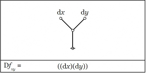
We did not yet go through the trouble to interpret this (first order) difference of conjunction fully, but were happy simply to evaluate it with respect to a single location in the universe of discourse, namely, at the point picked out by the singular proposition \(xy,\!\) that is, at the place where \(x = 1\!\) and \(y = 1.\!\) This evaluation is written in the form \(\operatorname{D}f|_{xy}\) or \(\operatorname{D}f|_{(1, 1)},\) and we arrived at the locally applicable law that is stated and illustrated as follows:

\(f(x, y) ~=~ xy ~=~ x ~\operatorname{and}~ y \quad \Rightarrow \quad \operatorname{D}f|_{xy} ~=~ \texttt{((} \operatorname{dx} \texttt{)(} \operatorname{d}y \texttt{))} ~=~ \operatorname{d}x ~\operatorname{or}~ \operatorname{d}y.\)

The picture shows the analysis of the inclusive disjunction \(\texttt{((} \operatorname{d}x \texttt{)(} \operatorname{d}y \texttt{))}\) into the following exclusive disjunction:

\(\operatorname{d}x ~\texttt{(} \operatorname{d}y \texttt{)} ~+~ \operatorname{d}y ~\texttt{(} \operatorname{d}x \texttt{)} ~+~ \operatorname{d}x ~\operatorname{d}y.\)

This resulting differential proposition may be interpreted to say "change \(x\!\) or change \(y\!\) or both". And this can be recognized as just what you need to do if you happen to find yourself in the center cell and desire a detailed description of ways to depart it.

Note 3

Last time we computed what will variously be called the difference map, the difference proposition, or the local proposition \(\operatorname{D}f_p\) for the proposition \(f(x, y) = xy\!\) at the point \(p\!\) where \(x = 1\!\) and \(y = 1.\!\)

In the universe \(U = X \times Y,\) the four propositions \(xy,~ x\texttt{(}y\texttt{)},~ \texttt{(}x\texttt{)}y,~ \texttt{(}x\texttt{)(}y\texttt{)}\) that indicate the "cells", or the smallest regions of the venn diagram, are called singular propositions. These serve as an alternative notation for naming the points \((1, 1),~ (1, 0),~ (0, 1),~ (0, 0),\!\) respectively.

Thus we can write \(\operatorname{D}f_p = \operatorname{D}f|p = \operatorname{D}f|(1, 1) = \operatorname{D}f|xy,\) so long as we know the frame of reference in force.

Sticking with the example \(f(x, y) = xy,\!\) let us compute the value of the difference proposition \(\operatorname{D}f\) at all 4 points.

o---------------------------------------o | | | x dx y dy | | o---o o---o | | \ | | / | | \ | | / | | \| |/ x y | | o=o-----------o | | \ / | | \ / | | \ / | | \ / | | \ / | | \ / | | @ | | | o---------------------------------------o | Df = ((x, dx)(y, dy), xy) | o---------------------------------------o

o---------------------------------------o | | | dx dy | | o---o o---o | | \ | | / | | \ | | / | | \| |/ | | o=o-----------o | | \ / | | \ / | | \ / | | \ / | | \ / | | \ / | | @ | | | o---------------------------------------o | Df|xy = ((dx)(dy)) | o---------------------------------------o

o---------------------------------------o | | | o | | dx | dy | | o---o o---o | | \ | | / | | \ | | / o | | \| |/ | | | o=o-----------o | | \ / | | \ / | | \ / | | \ / | | \ / | | \ / | | @ | | | o---------------------------------------o | Df|x(y) = (dx) dy | o---------------------------------------o

o---------------------------------------o | | | o | | | dx dy | | o---o o---o | | \ | | / | | \ | | / o | | \| |/ | | | o=o-----------o | | \ / | | \ / | | \ / | | \ / | | \ / | | \ / | | @ | | | o---------------------------------------o | Df|(x)y = dx (dy) | o---------------------------------------o

o---------------------------------------o | | | o o | | | dx | dy | | o---o o---o | | \ | | / | | \ | | / o o | | \| |/ \ / | | o=o-----------o | | \ / | | \ / | | \ / | | \ / | | \ / | | \ / | | @ | | | o---------------------------------------o | Df|(x)(y) = dx dy | o---------------------------------------o

The easy way to visualize the values of these graphical expressions is just to notice the following equivalents:

o---------------------------------------o | | | x | | o-o-o-...-o-o-o | | \ / | | \ / | | \ / | | \ / x | | \ / o | | \ / | | | @ = @ | | | o---------------------------------------o | (x, , ... , , ) = (x) | o---------------------------------------o

o---------------------------------------o | | | o | | x_1 x_2 x_k | | | o---o-...-o---o | | \ / | | \ / | | \ / | | \ / | | \ / | | \ / x_1 ... x_k | | @ = @ | | | o---------------------------------------o | (x_1, ..., x_k, ()) = x_1 · ... · x_k | o---------------------------------------o

Laying out the arrows on the augmented venn diagram, one gets a picture of a differential vector field.

o---------------------------------------o | | | dx dy | | ^ | | o | o | | / \ | / \ | | / \|/ \ | | /dy | dx\ | | /(dx) /|\ (dy)\ | | / ^ /`|`\ ^ \ | | / \``|``/ \ | | / /`\`|`/`\ \ | | / /```\|/```\ \ | | o x o`````o`````o y o | | \ \`````````/ / | | \ o---->```<----o / | | \ dy \``^``/ dx / | | \(dx) \`|`/ (dy)/ | | \ \|/ / | | \ | / | | \ /|\ / | | \ / | \ / | | o | o | | | | | dx | dy | | o | | | o---------------------------------------o

The Figure shows the points of the extended universe \(\operatorname{E}U = X \times Y \times \operatorname{d}X \times \operatorname{d}Y\) that satisfy the difference proposition \(\operatorname{D}f,\) namely, these:

\(\begin{array}{rcccc} 1. & x & y & dx & dy \\ 2. & x & y & dx & (dy) \\ 3. & x & y & (dx) & dy \\ 4. & x & (y) & (dx) & dy \\ 5. & (x) & y & dx & (dy) \\ 6. & (x) & (y) & dx & dy \end{array}\)

An inspection of these six points should make it easy to understand \(\operatorname{D}f\) as telling you what you have to do from each point of \(U\!\) in order to change the value borne by the proposition \(f(x, y).\!\)

Note 4

We have been studying the action of the difference operator \(\operatorname{D},\) also known as the localization operator, on the proposition \(f : X \times Y \to \mathbb{B}\) that is commonly known as the conjunction \(x \cdot y.\) We described \(\operatorname{D}f\) as a (first order) differential proposition, that is, a proposition of the type \(\operatorname{D}f : X \times Y \times \operatorname{d}X \times \operatorname{d}Y \to \mathbb{B}.\) Abstracting from the augmented venn diagram that illustrates how the models or satisfying interpretations of \(\operatorname{D}f\) distribute within the extended universe \(\operatorname{E}U = X \times Y \times \operatorname{d}X \times \operatorname{d}Y,\) we can depict \(\operatorname{D}f\) in the form of a digraph or directed graph, one whose points are labeled with the elements of \(U = X \times Y\) and whose arrows are labeled with the elements of \(\operatorname{d}U = \operatorname{d}X \times \operatorname{d}Y.\)

o---------------------------------------o | | | x · y | | | | o | | ^^^ | | / | \ | | (dx)· dy / | \ dx ·(dy) | | / | \ | | / | \ | | v | v | | x ·(y) o | o (x)· y | | | | | | | | dx · dy | | | | | | | | v | | o | | | | (x)·(y) | | | o---------------------------------------o | | | f = x y | | | | Df = x y · ((dx)(dy)) | | | | + x (y) · (dx) dy | | | | + (x) y · dx (dy) | | | | + (x)(y) · dx dy | | | o---------------------------------------o

Any proposition worth its salt, as they say, has many equivalent ways to look at it, any of which may reveal some unsuspected aspect of its meaning. We will encounter more and more of these alternative readings as we go.

Note 5

The enlargement or shift operator \(\operatorname{E}\) exhibits a wealth of interesting and useful properties in its own right, so it pays to examine a few of the more salient features that play out on the surface of our initial example, \(f(x, y) = xy.\!\)

A suitably generic definition of the extended universe of discourse is afforded by the following set-up:

\(\begin{array}{ccclll} \text{Let} & U & = & X_1 \times \ldots \times X_k. \'"`UNIQ-MathJax1-QINU`"' Amazing! =='"`UNIQ--h-7--QINU`"'Note 8== We have been contemplating functions of the type \(f : U \to \mathbb{B}\) and studying the action of the operators \(\operatorname{E}\) and \(\operatorname{D}\) on this family. These functions, that we may identify for our present aims with propositions, inasmuch as they capture their abstract forms, are logical analogues of scalar potential fields. These are the sorts of fields that are so picturesquely presented in elementary calculus and physics textbooks by images of snow-covered hills and parties of skiers who trek down their slopes like least action heroes. The analogous scene in propositional logic presents us with forms more reminiscent of plateaunic idylls, being all plains at one of two levels, the mesas of verity and falsity, as it were, with nary a niche to inhabit between them, restricting our options for a sporting gradient of downhill dynamics to just one of two: standing still on level ground or falling off a bluff. We are still working well within the logical analogue of the classical finite difference calculus, taking in the novelties that the logical transmutation of familiar elements is able to bring to light. Soon we will take up several different notions of approximation relationships that may be seen to organize the space of propositions, and these will allow us to define several different forms of differential analysis applying to propositions. In time we will find reason to consider more general types of maps, having concrete types of the form \(X_1 \times \ldots \times X_k \to Y_1 \times \ldots \times Y_n\) and abstract types \(\mathbb{B}^k \to \mathbb{B}^n.\) We will think of these mappings as transforming universes of discourse into themselves or into others, in short, as transformations of discourse. Before we continue with this intinerary, however, I would like to highlight another sort of differential aspect that concerns the boundary operator or the marked connective that serves as one of the two basic connectives in the cactus language for ZOL. For example, consider the proposition \(f\!\) of concrete type \(f : X \times Y \times Z \to \mathbb{B}\) and abstract type \(f : \mathbb{B}^3 \to \mathbb{B}\) that is written \(\texttt{(} x, y, z \texttt{)}\) in cactus syntax. Taken as an assertion in what Peirce called the existential interpretation, \(\texttt{(} x, y, z \texttt{)}\) says that just one of \(x, y, z\!\) is false. It is useful to consider this assertion in relation to the conjunction \(xyz\!\) of the features that are engaged as its arguments. A venn diagram of \(\texttt{(} x, y, z \texttt{)}\) looks like this: In relation to the center cell indicated by the conjunction \(xyz,\!\) the region indicated by \(\texttt{(} x, y, z \texttt{)}\) is comprised of the adjacent or bordering cells. Thus they are the cells that are just across the boundary of the center cell, as if reached by way of Leibniz's minimal changes from the point of origin, here, \(xyz.\!\) The same sort of boundary relationship holds for any cell of origin that one chooses to indicate. One way to indicate a cell is by forming a logical conjunction of positive and negative basis features, that is, by constructing an expression of the form \(e_1 \cdot \ldots \cdot e_k,\) where \(e_j = x_j ~\text{or}~ e_j = \texttt{(} x_j \texttt{)},\) for \(j = 1 ~\text{to}~ k.\) The proposition \(\texttt{(} e_1, \ldots, e_k \texttt{)}\) indicates the disjunctive region consisting of the cells that are just next door to \(e_1 \cdot \ldots \cdot e_k.\) Note 9 Consider what effects that might conceivably have practical bearings you conceive the objects of your conception to have. Then, your conception of those effects is the whole of your conception of the object. — Charles Sanders Peirce, "Issues of Pragmaticism", [CP 5.438] One other subject that it would be opportune to mention at this point, while we have an object example of a mathematical group fresh in mind, is the relationship between the pragmatic maxim and what are commonly known in mathematics as representation principles. As it turns out, with regard to its formal characteristics, the pragmatic maxim unites the aspects of a representation principle with the attributes of what would ordinarily be known as a closure principle. We will consider the form of closure that is invoked by the pragmatic maxim on another occasion, focusing here and now on the topic of group representations. Let us return to the example of the four-group \(V_4.\!\) We encountered this group in one of its concrete representations, namely, as a transformation group that acts on a set of objects, in this case a set of sixteen functions or propositions. Forgetting about the set of objects that the group transforms among themselves, we may take the abstract view of the group's operational structure, for example, in the form of the group operation table copied here: \(\cdot\) \(\operatorname{e}\) \(\operatorname{f}\) \(\operatorname{g}\) \(\operatorname{h}\) \(\operatorname{e}\) \(\operatorname{e}\) \(\operatorname{f}\) \(\operatorname{g}\) \(\operatorname{h}\) \(\operatorname{f}\) \(\operatorname{f}\) \(\operatorname{e}\) \(\operatorname{h}\) \(\operatorname{g}\) \(\operatorname{g}\) \(\operatorname{g}\) \(\operatorname{h}\) \(\operatorname{e}\) \(\operatorname{f}\) \(\operatorname{h}\) \(\operatorname{h}\) \(\operatorname{g}\) \(\operatorname{f}\) \(\operatorname{e}\) This operation table is abstractly the same as, or isomorphic to, the versions with the \(\operatorname{E}_{ij}\) operators and the \(\operatorname{T}_{ij}\) transformations that we discussed earlier. That is to say, the story is the same — only the names have been changed. An abstract group can have a multitude of significantly and superficially different representations. Even after we have long forgotten the details of the particular representation that we may have come in with, there are species of concrete representations, called the regular representations, that are always readily available, as they can be generated from the mere data of the abstract operation table itself. To see how a regular representation is constructed from the abstract operation table, pick a group element at the top of the table and "consider its effects" on each of the group elements listed on the left. These effects may be recorded in one of the ways that Peirce often used, as a logical aggregate of elementary dyadic relatives, that is, as a logical disjunction or sum whose terms represent the \(\operatorname{input} : \operatorname{output}\) pairs that are produced by each group element in turn. This forms one of the two possible regular representations of the group, specifically, the one that is called the post-regular representation or the right regular representation. It has long been conventional to organize the terms of this logical sum in the form of a matrix: Reading "\(+\!\)" as a logical disjunction: \(\mathrm{G} ~=~ \mathrm{e} + \mathrm{f} + \mathrm{g} + \mathrm{h}\) And so, by expanding effects, we get: \(\begin{matrix} \mathrm{G} & = & \mathrm{e}:\mathrm{e} & + & \mathrm{f}:\mathrm{f} & + & \mathrm{g}:\mathrm{g} & + & \mathrm{h}:\mathrm{h} \\ & + & \mathrm{e}:\mathrm{f} & + & \mathrm{f}:\mathrm{e} & + & \mathrm{g}:\mathrm{h} & + & \mathrm{h}:\mathrm{g} \\ & + & \mathrm{e}:\mathrm{g} & + & \mathrm{f}:\mathrm{h} & + & \mathrm{g}:\mathrm{e} & + & \mathrm{h}:\mathrm{f} \\ & + & \mathrm{e}:\mathrm{h} & + & \mathrm{f}:\mathrm{g} & + & \mathrm{g}:\mathrm{f} & + & \mathrm{h}:\mathrm{e} \end{matrix}\) More on the pragmatic maxim as a representation principle later. Note 10 The genealogy of this conception of pragmatic representation is very intricate. I'll sketch a few details that I think I remember clearly enough, subject to later correction. Without checking historical accounts, I won't be able to pin down anything approaching a real chronology, but most of these notions were standard furnishings of the 19th Century mathematical study, and only the last few items date as late as the 1920's. The idea about the regular representations of a group is universally known as "Cayley's Theorem", usually in the form: "Every group is isomorphic to a subgroup of Aut(S), the group of automorphisms of an appropriate set S". There is a considerable generalization of these regular representations to a broad class of relational algebraic systems in Peirce's earliest papers. The crux of the whole idea is this: | Consider the effects of the symbol, whose meaning you wish to investigate, | as they play out on "all" of the different stages of context on which you | can imagine that symbol playing a role. This idea of contextual definition is basically the same as Jeremy Bentham's notion of "paraphrasis", a "method of accounting for fictions by explaining various purported terms away" (Quine, in Van Heijenoort, page 216). Today we'd call these constructions "term models". This, again, is the big idea behind Schönfinkel's combinators {S, K, I}, and hence of lambda calculus, and I reckon you know where that leads. Note 11 Continuing to draw on the manageable materials of group representations, we examine a few of the finer points involved in regarding the pragmatic maxim as a representation principle. Returning to the example of an abstract group that we had before: \(\text{Klein Four-Group}~ V_4\) \(\cdot\) \(\operatorname{e}\) \(\operatorname{f}\) \(\operatorname{g}\) \(\operatorname{h}\) \(\operatorname{e}\) \(\operatorname{e}\) \(\operatorname{f}\) \(\operatorname{g}\) \(\operatorname{h}\) \(\operatorname{f}\) \(\operatorname{f}\) \(\operatorname{e}\) \(\operatorname{h}\) \(\operatorname{g}\) \(\operatorname{g}\) \(\operatorname{g}\) \(\operatorname{h}\) \(\operatorname{e}\) \(\operatorname{f}\) \(\operatorname{h}\) \(\operatorname{h}\) \(\operatorname{g}\) \(\operatorname{f}\) \(\operatorname{e}\) I presented the regular post-representation of the four-group V_4 in the following form: Reading "+" as a logical disjunction: G = e + f + g + h And so, by expanding effects, we get: G = e:e + f:f + g:g + h:h + e:f + f:e + g:h + h:g + e:g + f:h + g:e + h:f + e:h + f:g + g:f + h:e This presents the group in one big bunch, and there are occasions when one regards it this way, but that is not the typical form of presentation that we'd encounter. More likely, the story would go a little bit like this: I cannot remember any of my math teachers ever invoking the pragmatic maxim by name, but it would be a very regular occurrence for such mentors and tutors to set up the subject in this wise: Suppose you forget what a given abstract group element means, that is, in effect, 'what it is'. Then a sure way to jog your sense of 'what it is' is to build a regular representation from the formal materials that are necessarily left lying about on that abstraction site. Working through the construction for each one of the four group elements, we arrive at the following exegeses of their senses, giving their regular post-representations: e = e:e + f:f + g:g + h:h f = e:f + f:e + g:h + h:g g = e:g + f:h + g:e + h:f h = e:h + f:g + g:f + h:e So if somebody asks you, say, "What is g?", you can say, "I don't know for certain but in practice its effects go a bit like this: Converting e to g, f to h, g to e, h to f". I will have to check this out later on, but my impression is that Peirce tended to lean toward the other brand of regular, the "second", the "left", or the "ante-representation" of the groups that he treated in his earliest manuscripts and papers. I believe that this was because he thought of the actions on the pattern of dyadic relative terms like the "aftermath of". Working through this alternative for each one of the four group elements, we arrive at the following exegeses of their senses, giving their regular ante-representations: e = e:e + f:f + g:g + h:h f = f:e + e:f + h:g + g:h g = g:e + h:f + e:g + f:h h = h:e + g:f + f:g + e:h Your paraphrastic interpretation of what this all means would come out precisely the same as before. Note 12 Erratum Oops! I think that I have just confounded two entirely different issues: The substantial difference between right and left regular representations. The inessential difference between two conventions of presenting matrices. I will sort this out and correct it later, as need be. Note 13 Let me return to Peirce's early papers on the algebra of relatives to pick up the conventions that he used there, and then rewrite my account of regular representations in a way that conforms to those. Peirce describes the action of an "elementary dual relative" in this way: | [Let] A:B be taken to denote | the elementary relative which | multiplied into B gives A. | | Peirce, 'Collected Papers', CP 3.123. And though he is well aware that it is not at all necessary to arrange elementary relatives into arrays, matrices, or tables, when he does so he tends to prefer organizing dyadic relations in the following manner: | A:A A:B A:C | | | | B:A B:B B:C | | | | C:A C:B C:C | That conforms to the way that the last school of thought I matriculated into stipulated that we tabulate material: | e_11 e_12 e_13 | | | | e_21 e_22 e_23 | | | | e_31 e_32 e_33 | So, for example, let us suppose that we have the small universe \(\{ A, B, C \},\!\) and the 2-adic relation \(\mathrm{m} = {}^{\backprime\backprime} \text{mover of} \, {}^{\prime\prime}\) that is represented by this matrix: m = | m_AA (A:A) m_AB (A:B) m_AC (A:C) | | | | m_BA (B:A) m_BB (B:B) m_BC (B:C) | | | | m_CA (C:A) m_CB (C:B) m_CC (C:C) | Also, let \(\mathrm{m}\!\) be such that A is a mover of A and B, B is a mover of B and C, C is a mover of C and A. In sum: m = | 1 · (A:A) 1 · (A:B) 0 · (A:C) | | | | 0 · (B:A) 1 · (B:B) 1 · (B:C) | | | | 1 · (C:A) 0 · (C:B) 1 · (C:C) | For the sake of orientation and motivation, compare with Peirce's notation in CP 3.329. I think this much will serve to fix notation and set up the remainder of the discussion. Note 14 I am beginning to see how I got confused. It is common in algebra to switch around between different conventions of display, as the momentary fancy happens to strike, and I see that Peirce is no different in this sort of shiftiness than anyone else. A changeover appears to occur especially whenever he shifts from logical contexts to algebraic contexts of application. In the paper "On the Relative Forms of Quaternions" (CP 3.323), we observe Peirce providing the following sorts of explanation: | If X, Y, Z denote the three rectangular components of a vector, and W denote | numerical unity (or a fourth rectangular component, involving space of four | dimensions), and (Y:Z) denote the operation of converting the Y component | of a vector into its Z component, then | | 1 = (W:W) + (X:X) + (Y:Y) + (Z:Z) | | i = (X:W) - (W:X) - (Y:Z) + (Z:Y) | | j = (Y:W) - (W:Y) - (Z:X) + (X:Z) | | k = (Z:W) - (W:Z) - (X:Y) + (Y:X) | | In the language of logic (Y:Z) is a relative term whose relate is | a Y component, and whose correlate is a Z component. The law of | multiplication is plainly (Y:Z)(Z:X) = (Y:X), (Y:Z)(X:W) = 0, | and the application of these rules to the above values of | 1, i, j, k gives the quaternion relations | | i^2 = j^2 = k^2 = -1, | | ijk = -1, | | etc. | | The symbol a(Y:Z) denotes the changing of Y to Z and the | multiplication of the result by 'a'. If the relatives be | arranged in a block | | W:W W:X W:Y W:Z | | X:W X:X X:Y X:Z | | Y:W Y:X Y:Y Y:Z | | Z:W Z:X Z:Y Z:Z | | then the quaternion w + xi + yj + zk | is represented by the matrix of numbers | | w -x -y -z | | x w -z y | | y z w -x | | z -y x w | | The multiplication of such matrices follows the same laws as the | multiplication of quaternions. The determinant of the matrix = | the fourth power of the tensor of the quaternion. | | The imaginary x + y(-1)^(1/2) may likewise be represented by the matrix | | x y | | -y x | | and the determinant of the matrix = the square of the modulus. | | Charles Sanders Peirce, 'Collected Papers', CP 3.323. |'Johns Hopkins University Circulars', No. 13, p. 179, 1882. This way of talking is the mark of a person who opts to multiply his matrices "on the rignt", as they say. Yet Peirce still continues to call the first element of the ordered pair \((I:J)\!\) its "relate" while calling the second element of the pair \((I:J)\!\) its "correlate". That doesn't comport very well, so far as I can tell, with his customary reading of relative terms, suited more to the multiplication of matrices "on the left". So I still have a few wrinkles to iron out before I can give this story a smooth enough consistency. Note 15 I have been planning for quite some time now to make my return to Peirce's "Description of a Notation for the Logic of Relatives" (1870), and I can see that it's just about time to get down to it, so let this current bit of rambling inquiry function as the preamble to that. All we need at the present, though, is a way of telling what is substantial from what is inessential in the brook between symbolic conceits and dramatic actions that we find afforded by means of the pragmatic maxim. Back to our "subinstance", the example in support of our first example. I will try to reconstruct it in a less confusing way. Let us make up the model universe $1$ = A + B + C and the 2-adic relation n = "noder of", as when "X is a data record that contains a pointer to Y". That interpretation is not important, it's just for the sake of intuition. In general terms, the 2-adic relation n can be represented by this matrix: n = | n_AA (A:A) n_AB (A:B) n_AC (A:C) | | | | n_BA (B:A) n_BB (B:B) n_BC (B:C) | | | | n_CA (C:A) n_CB (C:B) n_CC (C:C) | Also, let n be such that A is a noder of A and B, B is a noder of B and C, C is a noder of C and A. Filling in the instantial values of the "coefficients" n_ij, as the indices i and j range over the universe of discourse: n = | 1 · (A:A) 1 · (A:B) 0 · (A:C) | | | | 0 · (B:A) 1 · (B:B) 1 · (B:C) | | | | 1 · (C:A) 0 · (C:B) 1 · (C:C) | In Peirce's time, and even in some circles of mathematics today, the information indicated by the elementary relatives (I:J), as I, J range over the universe of discourse, would be referred to as the "umbral elements" of the algebraic operation represented by the matrix, though I seem to recall that Peirce preferred to call these terms the "ingredients". When this ordered basis is understood well enough, one will tend to drop any mention of it from the matrix itself, leaving us nothing but these bare bones: n = | 1 1 0 | | | | 0 1 1 | | | | 1 0 1 | However the specification may come to be written, this is all just convenient schematics for stipulating that: n = A:A + B:B + C:C + A:B + B:C + C:A Recognizing !1! = A:A + B:B + C:C to be the identity transformation, the 2-adic relation n = "noder of" may be represented by an element !1! + A:B + B:C + C:A of the so-called "group ring", all of which just makes this element a special sort of linear transformation. Up to this point, we are still reading the elementary relatives of the form I:J in the way that Peirce reads them in logical contexts: I is the relate, J is the correlate, and in our current example we read I:J, or more exactly, n_ij = 1, to say that I is a noder of J. This is the mode of reading that we call "multiplying on the left". In the algebraic, permutational, or transformational contexts of application, however, Peirce converts to the alternative mode of reading, although still calling I the relate and J the correlate, the elementary relative I:J now means that I gets changed into J. In this scheme of reading, the transformation A:B + B:C + C:A is a permutation of the aggregate $1$ = A + B + C, or what we would now call the set {A, B, C}, in particular, it is the permutation that is otherwise notated as: ( A B C ) < > ( B C A ) This is consistent with the convention that Peirce uses in the paper "On a Class of Multiple Algebras" (CP 3.324-327). Note 16 | Consider what effects that might 'conceivably' | have practical bearings you 'conceive' the | objects of your 'conception' to have. Then, | your 'conception' of those effects is the | whole of your 'conception' of the object. | | Charles Sanders Peirce, | "Maxim of Pragmaticism", CP 5.438. We have been contemplating the virtues and the utilities of the pragmatic maxim as a hermeneutic heuristic, specifically, as a principle of interpretation that guides us in finding a clarifying representation for a problematic corpus of symbols in terms of their actions on other symbols or their effects on the syntactic contexts in which we conceive to distribute them. I started off considering the regular representations of groups as constituting what appears to be one of the simplest possible applications of this overall principle of representation. There are a few problems of implementation that have to be worked out in practice, most of which are cleared up by keeping in mind which of several possible conventions we have chosen to follow at a given time. But there does appear to remain this rather more substantial question: Are the effects we seek relates or correlates, or does it even matter? I will have to leave that question as it is for now, in hopes that a solution will evolve itself in time. Note 17 | Consider what effects that might 'conceivably' | have practical bearings you 'conceive' the | objects of your 'conception' to have. Then, | your 'conception' of those effects is the | whole of your 'conception' of the object. | | Charles Sanders Peirce, | "Maxim of Pragmaticism", CP 5.438. There a big reasons and little reasons for caring about this humble example. The little reasons we find all under our feet. One big reason I can now quite blazonly enounce in the fashion of this not so subtle subtitle: Obstacles to Applying the Pragmatic Maxim No sooner do you get a good idea and try to apply it than you find that a motley array of obstacles arise. It seems as if I am constantly lamenting the fact these days that people, and even admitted Peircean persons, do not in practice more consistently apply the maxim of pragmatism to the purpose for which it is purportedly intended by its author. That would be the clarification of concepts, or intellectual symbols, to the point where their inherent senses, or their lacks thereof, would be rendered manifest to all and sundry interpreters. There are big obstacles and little obstacles to applying the pragmatic maxim. In good subgoaling fashion, I will merely mention a few of the bigger blocks, as if in passing, and then get down to the devilish details that immediately obstruct our way. Obstacle 1. People do not always read the instructions very carefully. There is a tendency in readers of particular prior persuasions to blow the problem all out of proportion, to think that the maxim is meant to reveal the absolutely positive and the totally unique meaning of every preconception to which they might deign or elect to apply it. Reading the maxim with an even minimal attention, you can see that it promises no such finality of unindexed sense, but ties what you conceive to you. I have lately come to wonder at the tenacity of this misinterpretation. Perhaps people reckon that nothing less would be worth their attention. I am not sure. I can only say the achievement of more modest goals is the sort of thing on which our daily life depends, and there can be no final end to inquiry nor any ultimate community without a continuation of life, and that means life on a day to day basis. All of which only brings me back to the point of persisting with local meantime examples, because if we can't apply the maxim there, we can't apply it anywhere. And now I need to go out of doors and weed my garden for a time ... Note 18 | Consider what effects that might 'conceivably' | have practical bearings you 'conceive' the | objects of your 'conception' to have. Then, | your 'conception' of those effects is the | whole of your 'conception' of the object. | | Charles Sanders Peirce, | "Maxim of Pragmaticism", CP 5.438. Obstacles to Applying the Pragmatic Maxim Obstacle 2. Applying the pragmatic maxim, even with a moderate aim, can be hard. I think that my present example, deliberately impoverished as it is, affords us with an embarassing richness of evidence of just how complex the simple can be. All the better reason for me to see if I can finish it up before moving on. Expressed most simply, the idea is to replace the question of "what it is", which modest people know is far too difficult for them to answer right off, with the question of "what it does", which most of us know a modicum about. In the case of regular representations of groups we found a non-plussing surplus of answers to sort our way through. So let us track back one more time to see if we can learn any lessons that might carry over to more realistic cases. Here is is the operation table of V_4 once again: Table 1. Klein Four-Group V_4 o---------o---------o---------o---------o---------o | % | | | | | · % e | f | g | h | | % | | | | o=========o=========o=========o=========o=========o | % | | | | | e % e | f | g | h | | % | | | | o---------o---------o---------o---------o---------o | % | | | | | f % f | e | h | g | | % | | | | o---------o---------o---------o---------o---------o | % | | | | | g % g | h | e | f | | % | | | | o---------o---------o---------o---------o---------o | % | | | | | h % h | g | f | e | | % | | | | o---------o---------o---------o---------o---------o A group operation table is really just a device for recording a certain 3-adic relation, to be specific, the set of triples of the form <x, y, z> satisfying the equation x·y = z where · is the group operation. In the case of V_4 = (G, ·), where G is the "underlying set" {e, f, g, h}, we have the 3-adic relation L(V_4) c G x G x G whose triples are listed below: | <e, e, e> | <e, f, f> | <e, g, g> | <e, h, h> | | <f, e, f> | <f, f, e> | <f, g, h> | <f, h, g> | | <g, e, g> | <g, f, h> | <g, g, e> | <g, h, f> | | <h, e, h> | <h, f, g> | <h, g, f> | <h, h, e> It is part of the definition of a group that the 3-adic relation L c G^3 is actually a function L : G x G -> G. It is from this functional perspective that we can see an easy way to derive the two regular representations. Since we have a function of the type L : G x G -> G, we can define a couple of substitution operators: 1. Sub(x, <_, y>) puts any specified x into the empty slot of the rheme <_, y>, with the effect of producing the saturated rheme <x, y> that evaluates to x·y. 2. Sub(x, <y, _>) puts any specified x into the empty slot of the rheme <y, >, with the effect of producing the saturated rheme <y, x> that evaluates to y·x. In (1), we consider the effects of each x in its practical bearing on contexts of the form <_, y>, as y ranges over G, and the effects are such that x takes <_, y> into x·y, for y in G, all of which is summarily notated as x = {(y : x·y) : y in G}. The pairs (y : x·y) can be found by picking an x from the left margin of the group operation table and considering its effects on each y in turn as these run across the top margin. This aspect of pragmatic definition we recognize as the regular ante-representation: e = e:e + f:f + g:g + h:h f = e:f + f:e + g:h + h:g g = e:g + f:h + g:e + h:f h = e:h + f:g + g:f + h:e In (2), we consider the effects of each x in its practical bearing on contexts of the form <y, _>, as y ranges over G, and the effects are such that x takes <y, _> into y·x, for y in G, all of which is summarily notated as x = {(y : y·x) : y in G}. The pairs (y : y·x) can be found by picking an x from the top margin of the group operation table and considering its effects on each y in turn as these run down the left margin. This aspect of pragmatic definition we recognize as the regular post-representation: e = e:e + f:f + g:g + h:h f = e:f + f:e + g:h + h:g g = e:g + f:h + g:e + h:f h = e:h + f:g + g:f + h:e If the ante-rep looks the same as the post-rep, now that I'm writing them in the same dialect, that is because V_4 is abelian (commutative), and so the two representations have the very same effects on each point of their bearing. Note 19 | Consider what effects that might 'conceivably' | have practical bearings you 'conceive' the | objects of your 'conception' to have. Then, | your 'conception' of those effects is the | whole of your 'conception' of the object. | | Charles Sanders Peirce, | "Maxim of Pragmaticism", CP 5.438. So long as we're in the neighborhood, we might as well take in some more of the sights, for instance, the smallest example of a non-abelian (non-commutative) group. This is a group of six elements, say, G = {e, f, g, h, i, j}, with no relation to any other employment of these six symbols being implied, of course, and it can be most easily represented as the permutation group on a set of three letters, say, X = {A, B, C}, usually notated as G = Sym(X) or more abstractly and briefly, as Sym(3) or S_3. Here are the permutation (= substitution) operations in Sym(X): Table 2. Permutations or Substitutions in Sym_{A, B, C} o---------o---------o---------o---------o---------o---------o | | | | | | | | e | f | g | h | i | j | | | | | | | | o=========o=========o=========o=========o=========o=========o | | | | | | | | A B C | A B C | A B C | A B C | A B C | A B C | | | | | | | | | | | | | | | | | | | | | | | | | | | | | | | | | | v v v | v v v | v v v | v v v | v v v | v v v | | | | | | | | | A B C | C A B | B C A | A C B | C B A | B A C | | | | | | | | o---------o---------o---------o---------o---------o---------o Here is the operation table for S_3, given in abstract fashion: Table 3. Symmetric Group S_3 | _ | e / \ e | / \ | / e \ | f / \ / \ f | / \ / \ | / f \ f \ | g / \ / \ / \ g | / \ / \ / \ | / g \ g \ g \ | h / \ / \ / \ / \ h | / \ / \ / \ / \ | / h \ e \ e \ h \ | i / \ / \ / \ / \ / \ i | / \ / \ / \ / \ / \ | / i \ i \ f \ j \ i \ | j / \ / \ / \ / \ / \ / \ j | / \ / \ / \ / \ / \ / \ | ( j \ j \ j \ i \ h \ j ) | \ / \ / \ / \ / \ / \ / | \ / \ / \ / \ / \ / \ / | \ h \ h \ e \ j \ i / | \ / \ / \ / \ / \ / | \ / \ / \ / \ / \ / | \ i \ g \ f \ h / | \ / \ / \ / \ / | \ / \ / \ / \ / | \ f \ e \ g / | \ / \ / \ / | \ / \ / \ / | \ g \ f / | \ / \ / | \ / \ / | \ e / | \ / | \ / | ¯ By the way, we will meet with the symmetric group S_3 again when we return to take up the study of Peirce's early paper "On a Class of Multiple Algebras" (CP 3.324-327), and also his late unpublished work "The Simplest Mathematics" (1902) (CP 4.227-323), with particular reference to the section that treats of "Trichotomic Mathematics" (CP 4.307-323). Work Area | Consider what effects that might 'conceivably' | have practical bearings you 'conceive' the | objects of your 'conception' to have. Then, | your 'conception' of those effects is the | whole of your 'conception' of the object. | | Charles Sanders Peirce, | "Maxim of Pragmaticism", CP 5.438. By way of collecting a shot-term pay-off for all the work -- not to mention the peirce-spiration -- that we sweated out over the regular representations of V_4 and S_3 Table 2. Permutations or Substitutions in Sym_{A, B, C} o---------o---------o---------o---------o---------o---------o | | | | | | | | e | f | g | h | i | j | | | | | | | | o=========o=========o=========o=========o=========o=========o | | | | | | | | A B C | A B C | A B C | A B C | A B C | A B C | | | | | | | | | | | | | | | | | | | | | | | | | | | | | | | | | | v v v | v v v | v v v | v v v | v v v | v v v | | | | | | | | | A B C | C A B | B C A | A C B | C B A | B A C | | | | | | | | o---------o---------o---------o---------o---------o---------o problem about writing: e = e:e + f:f + g:g + h:h no recursion intended need for a work-around ways way explaining it away action on signs not objects math def of rep Document History 01. http://suo.ieee.org/ontology/msg04040.html 02. http://suo.ieee.org/ontology/msg04041.html 03. http://suo.ieee.org/ontology/msg04045.html 04. http://suo.ieee.org/ontology/msg04046.html 05. http://suo.ieee.org/ontology/msg04047.html 06. http://suo.ieee.org/ontology/msg04048.html 07. http://suo.ieee.org/ontology/msg04052.html 08. http://suo.ieee.org/ontology/msg04054.html 09. http://suo.ieee.org/ontology/msg04055.html 10. http://suo.ieee.org/ontology/msg04067.html 11. http://suo.ieee.org/ontology/msg04068.html 12. http://suo.ieee.org/ontology/msg04069.html 13. http://suo.ieee.org/ontology/msg04070.html 14. http://suo.ieee.org/ontology/msg04072.html 15. http://suo.ieee.org/ontology/msg04073.html 16. http://suo.ieee.org/ontology/msg04074.html 17. http://suo.ieee.org/ontology/msg04077.html 18. http://suo.ieee.org/ontology/msg04079.html 19. http://suo.ieee.org/ontology/msg04080.html